For my first post on Search Engine Land, I’ll start by quoting Ian Lurie:
Log file analysis is a lost art. But it can save your SEO butt!
Wise words.
However, getting the data we need out of server log files is usually laborious:
- Gigantic log files require robust data ingestion pipelines, a reliable cloud storage infrastructure, and a solid querying system
- Meticulous data modeling is also needed in order to convert cryptic, raw logs data into legible bits, suitable for exploratory data analysis and visualization
In the first post of this two-part series, I will show you how to easily scale your analyses to larger datasets, and extract meaningful SEO insights from your server logs.
All of that with just a pinch of Python and a hint of Google Cloud!
Here’s our detailed plan of action:
#1 – I’ll start by giving you a bit of context:
- What are log files and why they matter for SEO
- How to get hold of them
- Why Python alone doesn’t always cut it when it comes to server log analysis
#2 – We’ll then set things up:
- Create a Google Cloud Platform account
- Create a Google Cloud Storage bucket to store our log files
- Use the Command-Line to convert our files to a compliant format for querying
- Transfer our files to Google Cloud Storage, manually and programmatically
#3 – Lastly, we’ll get into the nitty-gritty of Pythoning – we will:
- Query our log files with Bigquery, inside Colab!
- Build a data model that makes our raw logs more legible
- Create categorical columns that will enhance our analyses further down the line
- Filter and export our results to .csv
In part two of this series (available later this year), we’ll discuss more advanced data modeling techniques in Python to assess:
- Bot crawl volume
- Crawl budget waste
- Duplicate URL crawling
I’ll also show you how to aggregate and join log data to Search Console data, and create interactive visualizations with Plotly Dash!
Excited? Let’s get cracking!
System requirements
We will use Google Colab in this article. No specific requirements or backward compatibility issues here, as Google Colab sits in the cloud.
Downloadable files
- The Colab notebook can be accessed here
- The log files can be downloaded on Github – 4 sample files of 20 MB each, spanning 4 days (1 day per file)
Be assured that the notebook has been tested with several million rows at lightning speed and without any hurdles!
Preamble: What are log files?
While I don’t want to babble too much about what log files are, why they can be invaluable for SEO, etc. (heck, there are many great articles on the topic already!), here’s a bit of context.
A server log file records every request made to your web server for content.
Every. Single. One.
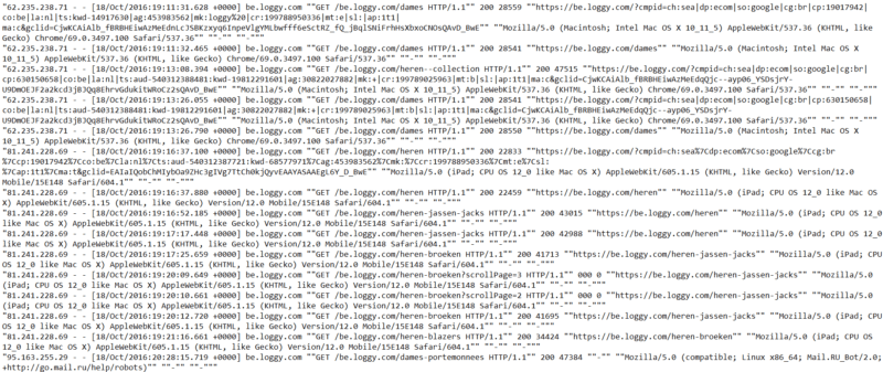
In their rawest forms, logs are indecipherable, e.g. here are a few raw lines from an Apache webserver:
Daunting, isn’t it?
Raw logs must be “cleansed” in order to be analyzed; that’s where data modeling kicks in. But more on that later.
Whereas the structure of a log file mainly depends on the server (Apache, Nginx, IIS etc…), it has evergreen attributes:
- Server IP
- Date/Time (also called timestamp)
- Method (GET or POST)
- URI
- HTTP status code
- User-agent
Additional attributes can usually be included, such as:
- Referrer: the URL that ‘linked’ the user to your site
- Redirected URL, when a redirect occurs
- Size of the file sent (in bytes)
- Time taken: the time it takes for a request to be processed and its response to be sent
Why are log files important for SEO?
If you don’t know why they matter, read this. Time spent wisely!
Accessing your log files
If you’re not sure where to start, the best is to ask your (client’s) Web Developer/DevOps if they can grant you access to raw server logs via FTP, ideally without any filtering applied.
Here are the general guidelines to find and manage log data on the three most popular servers:
We’ll use raw Apache files in this project.
Why Pandas alone is not enough when it comes to log analysis
Pandas (an open-source data manipulation tool built with Python) is pretty ubiquitous in data science.
It’s a must to slice and dice tabular data structures, and the mammal works like a charm when the data fits in memory!
That is, a few gigabytes. But not terabytes.
Parallel computing aside (e.g. Dask, PySpark), a database is usually a better solution for big data tasks that do not fit in memory. With a database, we can work with datasets that consume terabytes of disk space. Everything can be queried (via SQL), accessed, and updated in a breeze!
In this post, we’ll query our raw log data programmatically in Python via Google BigQuery. It’s easy to use, affordable and lightning-fast – even on terabytes of data!
The Python/BigQuery combo also allows you to query files stored on Google Cloud Storage. Sweet!
If Google is a nay-nay for you and you wish to try alternatives, Amazon and Microsoft also offer cloud data warehouses. They integrate well with Python too:
Amazon:
Microsoft:
Create a GCP account and set-up Cloud Storage
Both Google Cloud Storage and BigQuery are part of Google Cloud Platform (GCP), Google’s suite of cloud computing services.
GCP is not free, but you can try it for a year with $300 credits, with access to all products. Pretty cool.
Note that once the trial expires, Google Cloud Free Tier will still give you access to most Google Cloud resources, free of charge. With 5 GB of storage per month, it’s usually enough if you want to experiment with small datasets, work on proof of concepts, etc…
Believe me, there are many. Great. Things. To. Try!
You can sign-up for a free trial here.
Once you have completed sign-up, a new project will be automatically created with a random, and rather exotic, name – e.g. mine was “learned-spider-266010“!

Create our first bucket to store our log files
In Google Cloud Storage, files are stored in “buckets”. They will contain our log files.
To create your first bucket, go to storage > browser > create bucket:
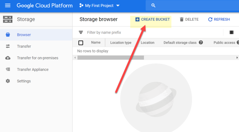
The bucket name has to be unique. I’ve aptly named mine ‘seo_server_logs’!
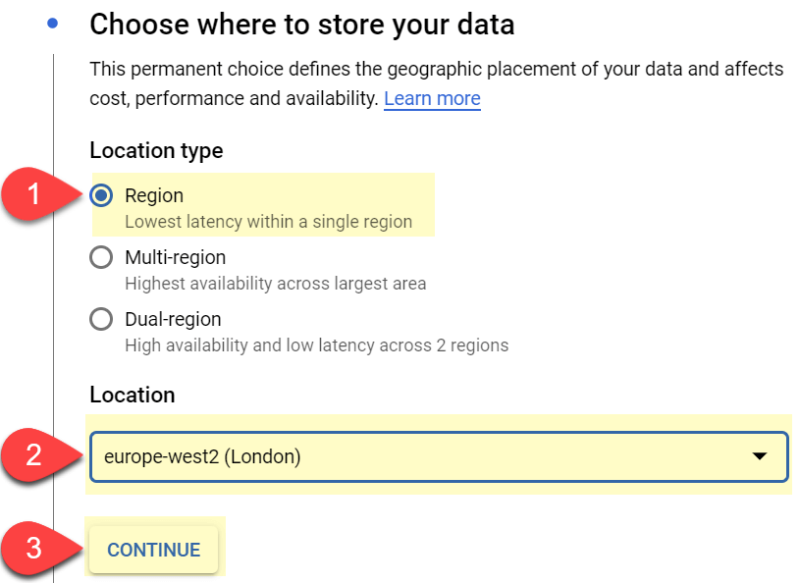
We then need to choose where and how to store our log data:
- #1 Location type – ‘Region’ is usually good enough.
- #2 Location – As I’m based in the UK, I’ve selected ‘Europe-West2’. Select your nearest location
- #3 Click on ‘continue’
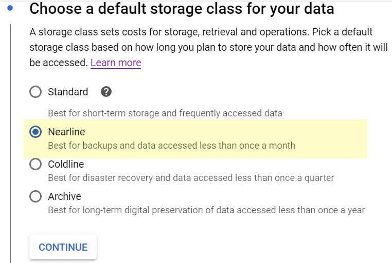
Default storage class: I’ve had good results with ‘nearline‘. It is cheaper than standard, and the data is retrieved quickly enough:
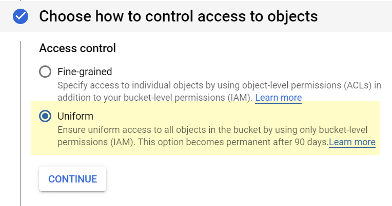
Access to objects: “Uniform” is fine:
Finally, in the “advanced settings” block, select:
- #1 – Google-managed key
- #2 – No retention policy
- #3 – No need to add a label for now
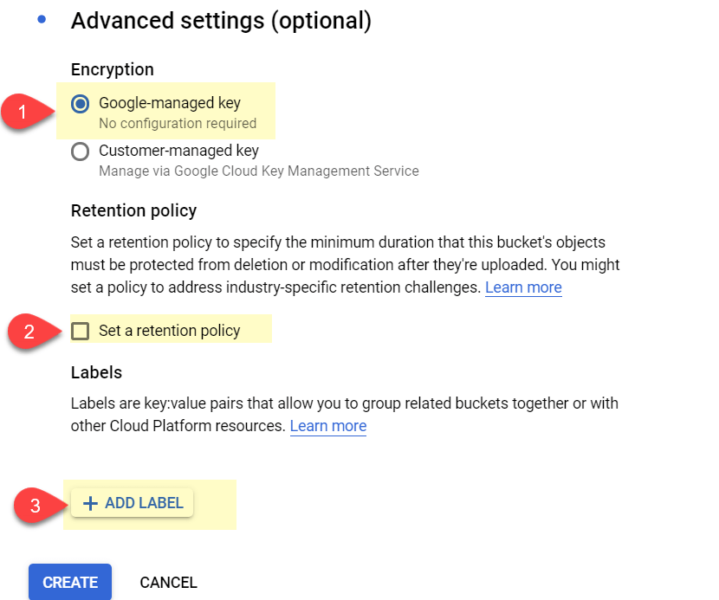
When you’re done, click “‘create.”
You’ve created your first bucket! Time to upload our log data.
Adding log files to your Cloud Storage bucket
You can upload as many files as you wish, whenever you want to!
The simplest way is to drag and drop your files to Cloud Storage’s Web UI, as shown below:
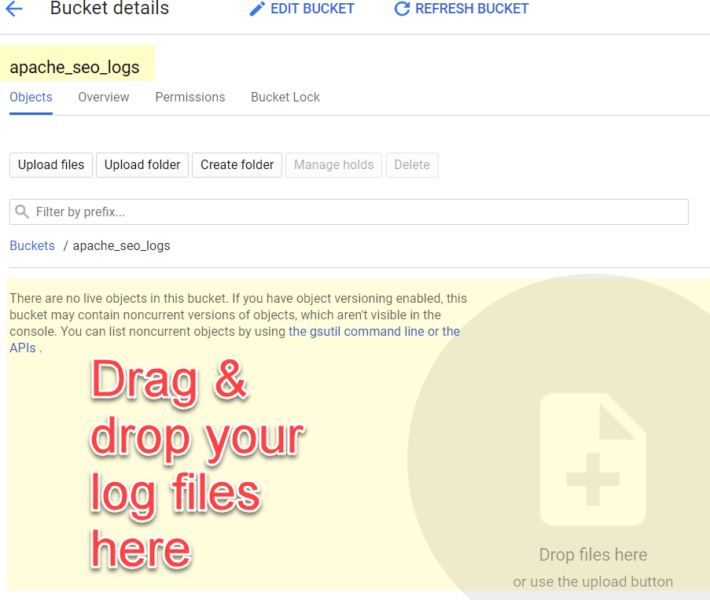
Yet, if you really wanted to get serious about log analysis, I’d strongly suggest automating the data ingestion process!
Here are a few things you can try:
- Cron jobs can be set up between FTP servers and Cloud Storage infrastructures:
- FTP managers like Cyberduck also offer automatic transfers to storage systems, too
- More data ingestion tips here (AppEngine, JSON API etc.)
A quick note on file formats
The sample files uploaded in Github have already been converted to .csv for you.
Bear in mind that you may have to convert your own log files to a compliant file format for SQL querying. Bigquery accepts .csv or .parquet.
Files can easily be bulk-converted to another format via the command line. You can access the command line as follows on Windows:
- Open the Windows Start menu
- Type “command” in the search bar
- Select “Command Prompt” from the search results
- I’ve not tried this on a Mac, but I believe the CLI is located in the Utilities folder
Once opened, navigate to the folder containing the files you want to convert via this command:
CD 'path/to/folder’
Simply replace path/to/folder with your path.
Then, type the command below to convert e.g. .log files to .csv:
for file in *.log; do mv "$file" "$(basename "$file" .*0).csv"; done
Note that you may need to enable Windows Subsystem for Linux to use this Bash command.
Now that our log files are in, and in the right format, it’s time to start Pythoning!
Unleash the Python
Do I still need to present Python?!
According to Stack Overflow, Python is now the fastest-growing major programming language. It’s also getting incredibly popular in the SEO sphere, thanks to Python preachers like Hamlet or JR.
You can run Python on your local computer via Jupyter notebook or an IDE, or even in the cloud via Google Colab. We’ll use Google Colab in this article.
Remember, the notebook is here, and the code snippets are pasted below, along with explanations.
Import libraries + GCP authentication
We’ll start by running the cell below:
It imports the Python libraries we need and redirects you to an authentication screen.
There you’ll have to choose the Google account linked to your GCP project.
Connect to Google Cloud Storage (GCS) and BigQuery
There’s quite a bit of info to add in order to connect our Python notebook to GCS & BigQuery. Besides, filling in that info manually can be tedious!
Fortunately, Google Colab’s forms make it easy to parameterize our code and save time.
The forms in this notebook have been pre-populated for you. No need to do anything, although I do suggest you amend the code to suit your needs.
Here’s how to create your own form: Go to Insert > add form field > then fill in the details below:

When you change an element in the form, its corresponding values will magically change in the code!
Fill in ‘project ID’ and ‘bucket location’
In our first form, you’ll need to add two variables:
- Your GCP PROJECT_ID (mine is ‘learned-spider-266010′)
- Your bucket location:
- To find it, in GCP go to storage > browser > check location in table
- Mine is ‘europe-west2′

Here’s the code snippet for that form:
Fill in ‘bucket name’ and ‘file/folder path’:
In the second form, we’ll need to fill in two more variables:

The bucket name:
- To find it, in GCP go to: storage > browser > then check its ‘name’ in the table
- I’ve aptly called it ‘apache_seo_logs’!
The file path:
- You can use a wildcard to query several files – Very nice!
- E.g. with the wildcarded path ‘Loggy*’, Bigquery would query these three files at once:
- Loggy01.csv
- Loggy02.csv
- Loggy03.csv
- Bigquery also creates a temporary table for that matter (more on that below)
Here’s the code for the form:
Connect Python to Google Cloud Storage and BigQuery
In the third form, you need to give a name to your BigQuery table – I’ve called mine ‘log_sample’. Note that this temporary table won’t be created in your Bigquery account.
Okay, so now things are getting really exciting, as we can start querying our dataset via SQL *without* leaving our notebook – How cool is that?!
As log data is still in its raw form, querying it is somehow limited. However, we can apply basic SQL filtering that will speed up Pandas operations later on.
I have created 2 SQL queries in this form:
- “SQL_1st_Filter” to filter any text
- “SQL_Useragent_Filter” to select your User-Agent, via a drop-down
Feel free to check the underlying code and tweak these two queries to your needs.
If your SQL trivia is a bit rusty, here’s a good refresher from Kaggle!
Code for that form:
Converting the list output to a Pandas Dataframe
The output generated by BigQuery is a two-dimensional list (also called ‘list of lists’). We’ll need to convert it to a Pandas Dataframe via this code:
Done! We now have a Dataframe that can be wrangled in Pandas!
Data cleansing time, the Pandas way!
Time to make these cryptic logs a bit more presentable by:
- Splitting each element
- Creating a column for each element
Split IP addresses
Split dates and times
We now need to convert the date column from string to a “Date time” object, via the Pandas to_datetime() method:
Doing so will allow us to perform time-series operations such as:
- Slicing specific date ranges
- Resampling time series for different time periods (e.g. from day to month)
- Computing rolling statistics, such as a rolling average
The Pandas/Numpy combo is really powerful when it comes to time series manipulation, check out all you can do here!
More split operations below:
Split domains
Split methods (Get, Post etc…)
Split URLs
Split HTTP Protocols
Split status codes
Split ‘time taken’
Split referral URLs
Split User Agents
Split redirected URLs (when existing)
Reorder columns
Time to check our masterpiece:
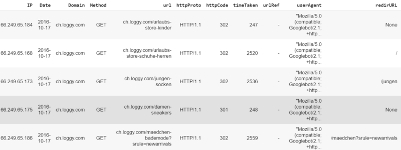
Well done! With just a few lines of code, you converted a set of cryptic logs to a structured Dataframe, ready for exploratory data analysis.
Let’s add a few more extras.
Create categorical columns
These categorical columns will come handy for data analysis or visualization tasks. We’ll create two, paving the way for your own experiments!
Create an HTTP codes class column
Create a search engine bots category column
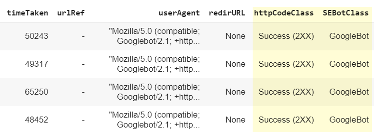
As you can see, our new columns httpCodeClass and SEBotClass have been created:
Spotting ‘spoofed’ search engine bots
We still need to tackle one crucial step for SEO: verify that IP addresses are genuinely from Googlebots.
All credit due to the great Tyler Reardon for this bit! Tyler has created searchtools.io, a clever tool that checks IP addresses and returns ‘fake’ Googlebot ones, based on a reverse DNS lookup.
We’ve simply integrated that script into the notebook – code snippet below:
Running the cell above will create a new column called ‘isRealGbot?:
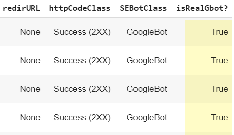
Note that the script is still in its early days, so please consider the following caveats:
- You may get errors when checking a huge amount of IP addresses. If so, just bypass the cell
- Only Googlebots are checked currently
Tyler and I are working on the script to improve it, so keep an eye on Twitter for future enhancements!
Filter the Dataframe before final export
If you wish to further refine the table before exporting to .csv, here’s your chance to filter out status codes you don’t need and refine timescales.
Some common use cases:
- You have 12 months’ worth of log data stored in the cloud, but only want to review the last 2 weeks
- You’ve had a recent website migration and want to check all the redirects (301s, 302s, etc.) and their redirect locations
- You want to check all 4XX response codes
Filter by date
Refine start and end dates via this form:

Filter by status codes
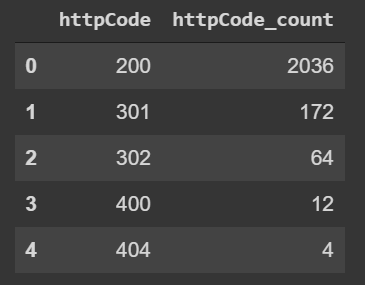
Check status codes distribution before filtering:
Code:
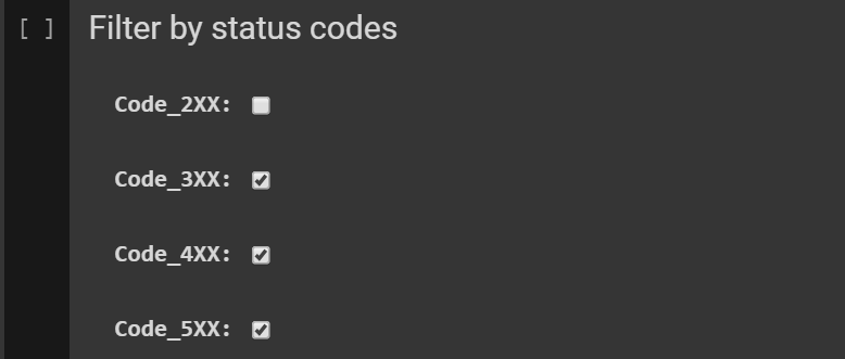
Then filter HTTP status codes via this form:
Related code:
Export to .csv
Our last step is to export our Dataframe to a .csv file. Give it a name via the export form:

Code for that last form:
Pat on the back if you’ve followed till here! You’ve achieved so much over the course of this article!
I cannot wait to take it to the next level in my next column, with more advanced data modeling/visualization techniques!
I’d like to thank the following people:
- Tyler Reardon, who’s helped me to integrate his anti-spoofing tool into this notebook!
- Paul Adams from Octamis and my dear compatriot Olivier Papon for their expert advice
- Last but not least, Kudos to Hamlet Batista or JR Oakes – Thanks guys for being so inspirational to the SEO community!
Please reach me out on Twitter if questions, or if you need further assistance. Any feedback (including pull requests! :)) is also greatly appreciated!
Happy Pythoning!
This year’s SMX Advanced will feature a brand-new SEO for Developers track with highly-technical sessions – many in live-coding format – focused on using code libraries and architecture models to develop applications that improve SEO. SMX Advanced will be held June 8-10 in Seattle. Register today.
Opinions expressed in this article are those of the guest author and not necessarily Search Engine Land. Staff authors are listed here.
