Last week, Hanapin hosted an Excel Extravaganza, which was a compilation of 3 Excel for PPC webinars in 3 days. On day 3, Lara and I discussed bidding methods with Excel. I specifically discussed bid tables and how to use Lookup functions to automatically pull bid changes from a bid table. We discussed how to write lookup functions, specifically the Index + Match, but I want to follow up with a quick guide to troubleshooting Lookup functions.
It’s easy to make mistakes when writing new functions, and receiving errors in Excel is often what intimidates people from using Excel more often. My goal with this post is to make it easy to find and correct your mistakes when writing lookup functions in Excel so that you’re not afraid to use them! (If you didn’t catch the webinars, check them out. If you want a written explanation of the Index + Match, check out this post.)
Index
As I mentioned, the bid table method I taught in the webinar focused on the Index and Match functions. When used alone, the Index function is relatively simple. There’s only one main error I see people make when writing an Index function without a Match:

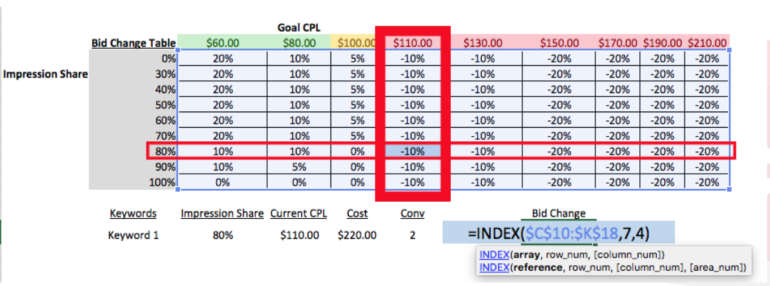
In the example above (from the webinar), you can see that we have a simple Index function with three arguments: array, row_num, column_num. The Array argument is the table of data from which we want to pull bid change percentages. The most common error I see is that people forget to anchor ($A$1) their Array. When that happens, the first cell with this Index function works fine. However, if you copy that function down a full column, you’ll begin to get the wrong answers and eventually you’ll receive errors. When the Array is NOT anchored, the cell references move in the same direction as the function that’s being copied down or across an Excel worksheet.
Just remember: in 95% of Excel functions, you should anchor ranges of data.
Index + Match
As a reminder, here is the definition and the makeup of a Match function:
When we add the Match function into an Index, it naturally becomes more difficult to troubleshoot as the number of arguments has doubled or even tripled. Here are the most common errors I see with Match functions:
Both the Index and Match functions have an Array argument, which often leads people to believe those should be the exact same range of data. This is WRONG. The Array in a Match can ONLY be one row OR one column of data. The Array for and Index is usually multiple rows and columns.
The second-most common mistake I see is that people forget the third argument: Match Type. This argument is tricky! It’s in brackets because it’s optional. However, the default that Excel uses if the argument is “1”, which is not always what the user intended. Below are the options we’re given for the Match Type argument.
VLookup and HLookup Functions
I did not cover the VLookup or HLookup functions in the webinar, but they’re often used instead of the Index + Match functions. They’re less flexible than the Index+Match, so there are some instances where Index+Match is the ONLY lookup function that will work. However, many people don’t run into those scenarios and find the VLookup and HLookup functions easier to understand. Here are the most common pitfalls I see with these lookup functions:
The “V” in VLookup stands for “vertical”. This is key to understanding the arguments of this function. The Lookup_Value MUST be located in the first (vertical) column of the array. The example below shows an example of this mistake.
The Lookup_Value argument shows that I’m looking for “Keyword 2”. For this function to work, the keywords need to be in the FIRST column of the array I’m using. However, I’m using an array from A-E, meaning the first column is the campaign name. When the function can’t find the value you’re looking for, you’ll get an “#N/A” error.
HLOOKUP
The HLookup is nearly identical to the VLookup, except that it’s meant for horizontal data tables (hence the “H”). That means the most common errors are basically the same. The Lookup_Value MUST be located in the first (horizontal) row of the array.
In addition, it’s easy for people to forget the optional fourth argument of an Hlookup or a Vlookup: the range_lookup. The range_lookup argument has two options: True or False. When this argument isn’t specified by the user, Excel defaults to True. The True option means your function will look for an APPROXIMATE match to the lookup_value you’ve specified. If you’re looking for an exact keyword, exact number, or an exact piece of text you need to use False.
Conclusion
Lookup functions can be very helpful for PPC analysis and PPC automation. However, it’s easy to get discouraged from using Excel when we run into errors. I hope this post helps you all to troubleshoot your Lookup functions a little faster so you don’t refrain from using them!