Forecasting sales is useful for many reasons, such as inventory management, investor relations, and setting expense and marketing budgets. But producing accurate forecasts can be confusing. In this post, I’ll explain how to generate forecasts using Microsoft Excel.
Gathering Data
To start, identify the objective. What is the purpose of your analysis? Then gather data and run a forecasting model.
First, establish the timeline. Are you looking to predict the next 12 months, the next five years, or the next 30 days? For a 12-month analysis, it is best to have at least three years of data to establish seasonality trends. If you only have a few months of data, use it to estimate the next 30 days or so.
Next, gather the data based on the type of forecast.
| Type of Forecast | Data Required |
|---|---|
| Overall sales | Total sales volume by years, months, or days. |
| Sales for each product | Sales volume by product name or type. |
| Sales by geography | Sales volume by desired region (i.e., country, state). |
| Sales by marketing channel | Sales volume by channel, such as Facebook, organic search, Google Ads. |
You can predict sales for most key metrics as long as you have the historical data.
Methodology
Once you have the data in a table form, use the TREND function in Excel for your predictions, as follows.
= TREND(Historical Sales, Historical Timeline, Forecast Timeline)
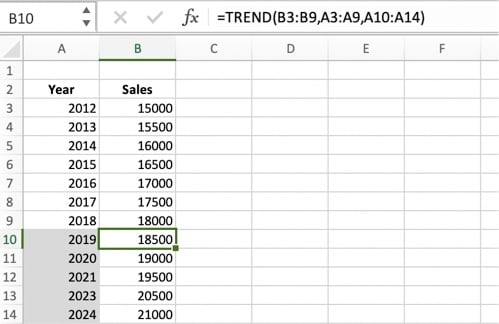
In the Excel screenshot, below, the formula is:
=TREND(B3:B9,A3:A9,A10:A14)

Once you have the data in a table form, use the TREND function in Excel for forecasts. Click image to enlarge.
Note that the TREND formula in Excel is linear. But, for most ecommerce companies, sales are not consistent throughout the year. Sales in October, November, and December can account for most of the annual total. Building seasonality effects into a forecasting model is a bit more complicated.
- Step 1. Calculate the average historical sales per month.
- Step 2. Compute a seasonality adjustment for each month.
- Step 3. Multiply the seasonality adjustment times the average monthly total sales to get your forecast.
For example, assume we have annual sales data for the past three years. We have calculated the average sales per month for each of those years (2016 through 2018) and assigned a seasonality adjustment for each month. Here’s a screenshot for 2018.
Average 2018 monthly sales were $6,638. Sales in October, November, and December exceeded the average by, respectively, 98 percent, 105 percent, and 301 percent. Click image to enlarge.
Next, we apply the TREND function to forecast average 2019 monthly sales — $6,924 in this example.
Then we apply the monthly seasonality adjustment to the 2019 forecast.
Applying the seasonality adjustments to the 2019 forecast alters projected monthly totals. Click image to enlarge.
You can apply the TREND function and seasonality techniques to products, marketing channel, geography, and so on.
Adding Assumptions
Sometimes it’s helpful to add assumptions to forecasts, such as an increase in sales from product launches or promotions.
Here’s an example. Say a new product will launch in April. You anticipate it will contribute $50 in sales for that month and will slowly increase by 5 percent monthly. However, certain historical promotions have generated a 20 percent increase in monthly sales, and you plan on using those promotions for the new product in February and August.
Thus, our Excel spreadsheet now includes a new row for the anticipated 20 percent increase in February and August, which produces new predictions for 2019.
Adding assumptions can make forecasts more accurate. In this example, the forecast includes the anticipated impact of marketing promotions in February and August. Click image to enlarge.
Basic vs. Complex
The examples above are simplified methods of basic forecasting. More complicated models could include additional assumptions, variables beyond seasonality, and multiple product types. Advanced models could also consider inventory levels and competitor initiatives, for instance.
The same forecasting methods can predict expenses (such as estimated pay-per-click costs), inventory level, product demand, and hiring needs. As long as you have relevant data, you can usually build a forecasting model.